To solve the data centre location problem, we will design a cost function that gives a value for every longitude and latitude, representing how suitable a given coordinate is for a data centre (high values indicate poor locations and low values indicate good locations). This cost function also utilises publicly available data to guide our location search. We want locations that optimise performance, minimise latency, operate smoothly, and consume energy efficiently. To do this, we shall consider several variables and datasets.
We consider five different sets of data for our cost function. The first two are based on electricity (obviously important for data centres), the next one is based on water sources (we need water for cooling in data centres), the next one is based on population, as this gives an idea of service coverage for data transmission. We also assume this is a good approximation of where telecommunications networks will be prevalent (low latency). We make this assumption as telecommunications network data doesn't seem to be easily accessible to the public (proprietary datasets). Finally, we consider temperature, as we don't want data centres operating in hot areas of Australia (more cooling is required). For the following functions, p is our longitude and latitude coordinate.
Here we are summing over all power stations that are within a 300 km radius of our coordinate. Capacity is the output of the power station (we estimated this output based on how the power was generated). \(w_{green,i}\) is a coefficient we multiply by, based on whether the power generation is green or not (1.2 if renewable, and 1.0 if not). Finally, we have \(d_{i}\), which is the distance from our point to the power station (we add 1 to it in the denominator to avoid dividing by zero and generating extreme values for distances < 1).
Here, \(V_{i}\) is the voltage that the substations regulate, and again \(d_{i}\) is the distance to the substation (we again sum over all substations within a 300 km radius of our coordinate). Note that we take the natural logarithm of this sum, as during testing we found these values to be abnormally large compared to the other parts of our cost function.
In this term, we again sum over all lakes within a 300 km radius. However, we did a lot of preprocessing to exclude water sources that are not perennial (not full-year-round), and also to only consider large water sources. Here we sum over the surface area (\(A_{i}\)) of the water sources (a good indication of water availability), divided by the distance to those water sources.
Here, we only consider the closest population centre to our coordinate. We then take the population and divide it by the area that the population centre covers (normalisation). We use this exponential function to give high scores for low population density. The hyperparameters (200 and 0.1) were chosen because they give this part of the cost function values that align well with the rest of the function.
Here, 200 is a hyperparameter (again chosen because it aligns well with the other values of the cost function), and we are just looking at the closest temperature recording station. The average maximum temperature is used, as this is a good estimate of the worst-case scenario in temperature for the data centre. We also add the longitude, as increasing it tends to correlate with an increase in temperature. Again, we divide by the distance to the station that recorded the temperatures (plus 1).
Finally, we sum all these costs together, multiplying each by coefficients which describe the importance of each term to the cost (v, w, x, y, z) to get the cost of placing a data centre at a certain location. The coefficients are 35, 15, 10, 5 and 15 respectively (electricity consumption is very important, temperature and water sources are important, and population density is less important — it was a weak assumption we made due to lack of access to better data).

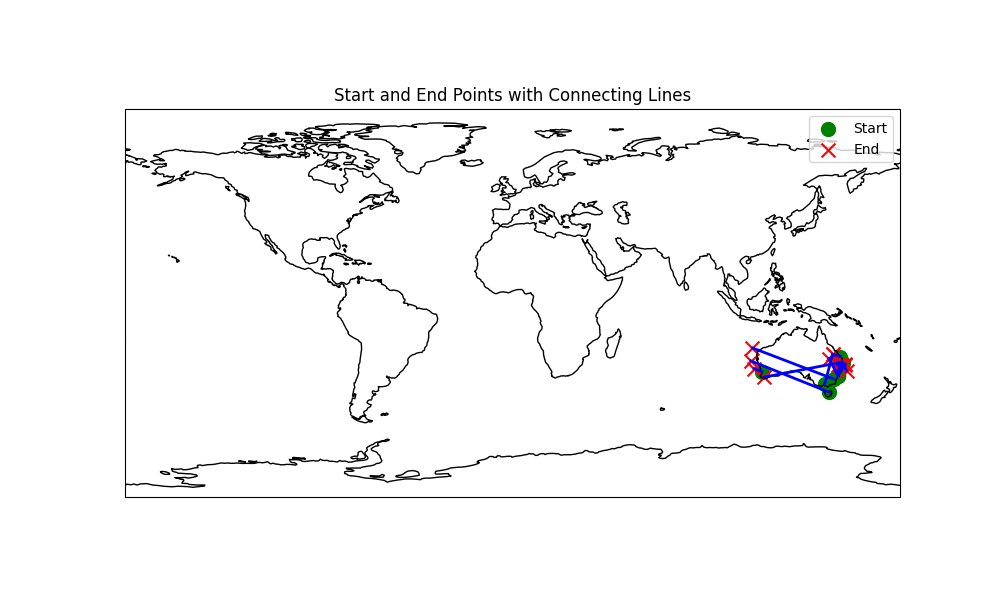
Running L-BFGS to optimise our cost function with starting values at major Australian cities, we see that the optimisation tends to move to coastal regions. This is expected, as these regions contain the ideal climate and resources needed for data centres.

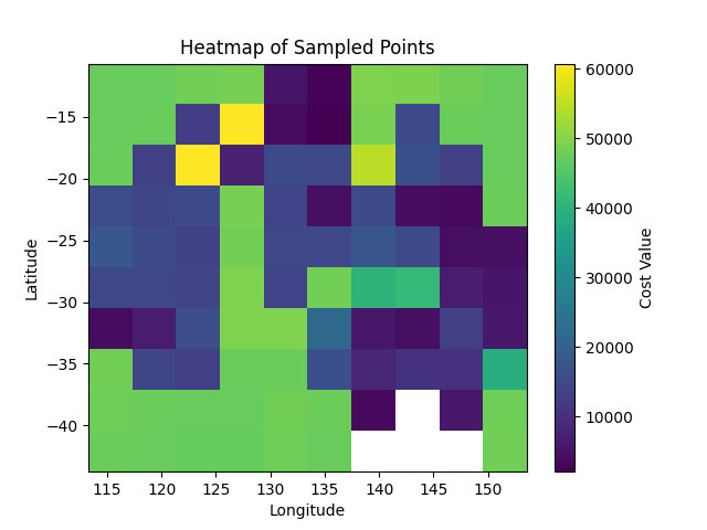
Looking at the heat map for values of the cost function across Australia, we again see that coastal regions have lower cost (except in some places up north that lack infrastructure). Some particularly promising locations appear to be around Perth, South East Queensland, Darwin, and Adelaide.
Moving forward with this model, we would need to integrate smart grid data for real-time energy usage across Australia to optimise data centre performance (possibly training an RNN or transformer model to predict time series data using AI). We didn’t have access to good data for this, so we didn’t integrate it into the model. We could also integrate information about fibre optic infrastructure if we had access to it (proprietary data). In terms of regulations, we can examine the locations our current model selected and seek expert opinions about how the laws and regulations of each location will affect building and maintaining data centres, and how they will affect operations. Finally, in the future, we may wish to consider data about floods and bushfires (natural disasters that regularly affect Australia) to further improve the performance of our cost function.