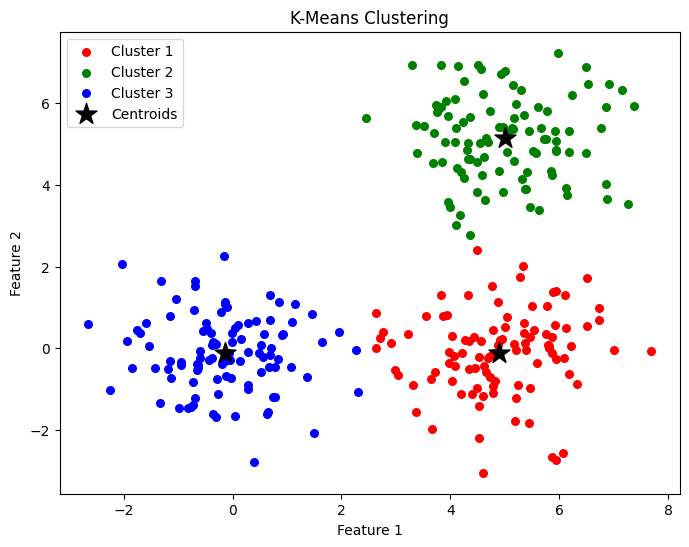
Figure: Plot of the clusters and the learned centroids
In this chapter we will have a look at other methods in machine learning which don't quite fall under the umbrella of regression or classification, or that extend some of the ideas discussed in previous articles. The first algorithm we will be looking at is K-Means, which is used to cluster data. It is an unsupervised algorithm, meaning we don't require prior knowledge of class labels. The algorithm will find clusters of data that belong to different classes, k (which we set) classes to be exact. We are given our data, \(X=(x_{1},...,x_{n})\) where each \(x_{i}\in\mathbb{R}^{d}\) and we want to partition them into k clusters \(C=\{C_{1},...,C_{k}\}\) each with a centroid \(\mu_{j}\in\mathbb{R}^{d}\). The overall goal of k-means is to minimise the total within-cluster sum of squares:
We solve this through an iterative procedure. We start by randomly initialising \(k\) data points as the initial centroids (\(\mu_{1}^{(0)},...,\mu_{k}^{(0)}\)). We then assign each data point \(x_{i}\) to the nearest centroid based on minimal distance, i.e.:
We then update our centroids by calculating the mean of all the points assigned to that cluster:
We then repeat assigning each data point to the nearest centroid and recalculating the new centroids until either a maximum number of iterations is reached or:
Where \(\epsilon\) is a tolerance parameter (stop when updating centroids doesn't change them very much). Implementing this in code we get:
class KMeans:
    def __init__(self, n_clusters=3, max_iters=100, tol=1e-4, random_state=None):
        self.n_clusters = n_clusters
        self.max_iters = max_iters
        self.tol = tol
        self.random_state = random_state
        self.centroids = None

    def fit(self, X):
        if self.random_state:
            np.random.seed(self.random_state)

        # Initialize centroids randomly from data points
        random_indices = np.random.choice(len(X), self.n_clusters, replace=False)
        self.centroids = X[random_indices]

        for i in range(self.max_iters):
            # Assign clusters
            clusters = self._assign_clusters(X)

            # Compute new centroids
            new_centroids = np.array([X[clusters == k].mean(axis=0) if len(X[clusters == k]) > 0 else self.centroids[k]
                                      for k in range(self.n_clusters)])

            # Check for convergence
            if np.all(np.linalg.norm(new_centroids - self.centroids, axis=1) < self.tol):
                break

            self.centroids = new_centroids

    def _assign_clusters(self, X):
        # Compute distances to centroids
        distances = np.linalg.norm(X[:, np.newaxis] - self.centroids, axis=2)
        # Assign each point to closest centroid
        return np.argmin(distances, axis=1)

    def predict(self, X):
        return self._assign_clusters(X)
Training it on some randomly generated data and setting the number of centroids to three we get:
In order to choose the best \(k\) there are a few methods. The first obvious one is using domain knowledge, e.g. if we were to train it on the iris dataset we would choose \(k=3\) as there are three species. Another method is to plot the \(WCSS(k)\) against \(k\) and choose the \(k\) at which \(WCSS(k)\) doesn't increase by much. The final method I'll discuss is the silhouette score which measures how well a point fits into its cluster compared to others. The silhouette score for a single data point \(x_{i}\) is:
Where \(a(i)\) is the average distance of \(x_{i}\) to other points in its own cluster and \(b(i)\) is the lowest average distance of \(x_{i}\) to points in any other cluster. If \(s(i)\) is close to 1 it is well clustered, if it is close to 0 the point is on the boundary and if it is less than 0 the point is misclassified. We then compute the average score for all points and choose the \(k\) that gives the highest average silhouette. There are a few other ways to choose \(k\) but thats all I'll cover here.