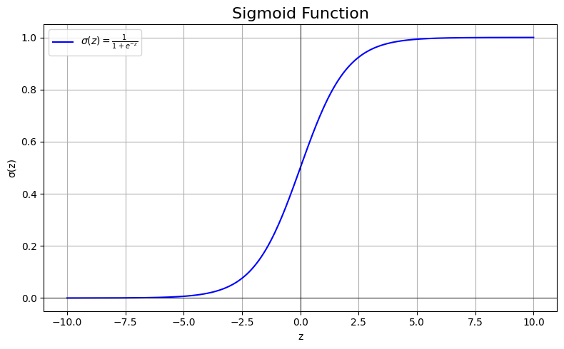
Figure: Plot of the sigmoid function
We now move onto our first classification model, logisitic regression. In this model we only have two classes which we will label with 0 and 1. We can then model the probability that for a given piece of data that we see it is of class 1 as follows:
This is the sigmoid function and we'll see a lot more of it later on when we work on neural networks (and also in the next tutorial when we extend logistic regression to multiple classes). This is because when we plot it we see that it acts as a "threshold" with mostly taking values close to 0 or 1 but in the middle it curves up from 0 to 1.
For this problem we will use a binary cross entropy loss function (BCE). We will use this as we are modelling probability distributions (\(P(y=1|x)\) and \(P(y=0|x)=1-P(y=1|x)\)) and BCE measures the average number of bits (0, 1) needed to identify an event drawn from the estimated distribution (\(P(y=1|x)\)) rather than the true distribution, whatever that may be. This is related to entropy from information theory but I won't go in depth about it here. BCE is defined as:
In our case \(p_i=\sigma(x_{i}^{T}\beta)\). We can also rewrite our model to output all predictions as vector through matrix notation (noting that we add a 1's column for our bias) as such:
We can now perform optimisation the way we normally do through taking the gradient:
I won't give a proof of it here but you can find a proof of this fact here, or you can try and prove it yourself 😀. If we try and set the gradient to zero and solve for \(\beta\) we will quickly realise there is no closed form solution and hence we can use gradient descent to find the minimum.
Before we implement it one thing to note is that the sigmoid function can sometimes run into overflow errors so we only compute \(\exp(-z)\) where \(z\geq0\) and compute \(\exp(z)\) where \(z<0\). To ensure this we use two experessions \(\frac{1}{1+e^{-z}}\) and \(\frac{e^{z}}{1+e^{z}}\) which are equal to each other (multiply the first expression by \(\frac{e^{z}}{e^{z}}\)).
    import numpy as np

    def sigmoid(z):
        z = np.array(z)  # ensure it's an array for element-wise ops
        result = np.empty_like(z, dtype=np.float64)

        pos_mask = z >= 0
        neg_mask = ~pos_mask

        result[pos_mask] = 1 / (1 + np.exp(-z[pos_mask]))
        result[neg_mask] = np.exp(z[neg_mask]) / (1 + np.exp(z[neg_mask]))

        return result

    def logistic_loss(X, y, beta):
        m = len(y)
        z = X @ beta
        p = sigmoid(z)
        epsilon = 1e-15  # to avoid log(0)
        return -np.mean(y * np.log(p + epsilon) + (1 - y) * np.log(1 - p + epsilon))

    def logistic_gradient(X, y, beta):
        m = len(y)
        p = sigmoid(X @ beta)
        return (1 / m) * (X.T @ (p - y))

    def logistic_regression(X, y, lr=0.1, epochs=1000):
        X = np.c_[np.ones(X.shape[0]), X]  # Add bias term
        beta = np.zeros(X.shape[1])

        for _ in range(epochs):
            grad = logistic_gradient(X, y, beta)
            beta -= lr * grad

        return beta

    def predict(X, beta, threshold=0.5):
        X = np.c_[np.ones(X.shape[0]), X]  # Add bias
        return sigmoid(X @ beta) >= threshold
In the colab notebook we then train our model on the breast cancer dataset (predict whether or not a patient has breast cancer) and we get an accuracy of 91.56%.