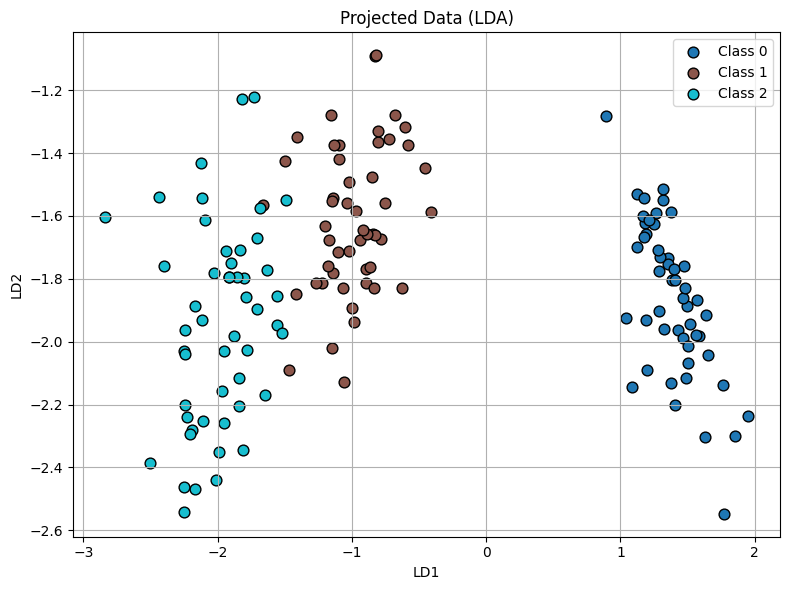
Figure: Plot of iris data after projection
LDA is an interesting topic in machine learning as it can not only be used for classification but also for dimensionality reduction. We will see how both approaches to this problem work and the connection between them. In the setup of LDA we are given a set of samples \(x_{1},...,x_{n}\) and class labels \(y_{1},...,y_{n}\) (there are K different classes). It also assumes that all class-conditional distributions (\(p(x|y=k)\)) are distributed according to a multivariate gaussian (as seen below, also note that \(|\cdot|\) is the determinant), all classes share the same covariance matrix (\(\Sigma\)) and each class has a prior probability \(\pi_{k}=\frac{n_{k}}{n}\), where \(n_{k}\) is the number of samples from class k.
We can now find the probability of a sample belonging to a class using bayes theorem:
As \(p(x)\) is the same for all classes the class with the highest numerator will be chosen (ignore p(x)). Taking the log of the numerator (as its easier to work with) we get our discriminant function:
Expanding this out and getting rid of terms that will be constant for all classes we get:
Expanding this out and again dropping terms that will be constant for all classes we get:
This is our discriminant function, I'll also leave the steps I've skipped as an exercise for you. We can also see why it's called LINEAR discriminant analysis as we can rewrite our discriminant function as:
To classify we now just choose the k for which \(\delta_{k}(x)\) returns the highest value, which is the following rule:
That was clasification, we now move onto dimensionality reduction. Our goal is to project our data into a subspace in which the classes are best seperated. We can start this by calculating the within class "scatter" \(S_{w}\) and between class "scatter" \(S_{b}\). You can think of this as how far away the samples are from the class means and how far the class means are from each other. We can calculate them as:
Here \(\mu_{k}\) is the sample mean of the kth class, \(\mu\) is the overall sample mean and \(\sum_{x_{i}\in C_{k}}\) means sum over all the samples from the kth class. Now we want to construct an objective function that achieves our goal. First we define a projection matrix \(W=[w_1,...,w_{k-1}]\) (\(W\in\mathbb{R}^{d\times(K-1)}\)) as a matrix of what we later see are eigenvectors that correspond to the largest eigenvalues. With \(W\) we can now measure the spread between class means after projection with \(|W^{T}S_{B}W|\) and the spread within each class after projection with \(|W^{T}S_{B}W|\). Recall that the determinant gives the signed volume of the n-dimensional parallelepiped and hence we are getting a measure of the within class and between class spread after projection. As we want the seperate classes far apart but the samples from the same class close we want to make the volume of the n-dimensional parallelepiped for within class small and the between class large which can be achieved by maximising the following ratio.
Reframing it as an optimisation problem we get:
As we are solving for eigenvectors the problem becomes more tractable if we first reduce it to one vector, namely we want to find:
Before we attempt to solve this optmisation problem we must first note some properties of the objective function. First it is invariant to scaling which we will now prove (c is a constant).
As it is invariant to scaling there is no finite minimum or maximum it just keeps growing/shrinking with the scale of \(w_{i}\). We also have that the ratio is non-linear. So, instead of optimizing over all possible \(w_{i}\), we fix the scale of the denominator to 1 in order to remove this ambiguity. This gives us the following optimisation problem:
In this problem we are finding the direction \(w_{i}\) that makes the numerator as big as possible, without letting the denominator grow. We also see that we can solve this using lagrange multipliers which gives us the following loss function:
Taking the gradient we get:
Setting to zero and rearranging we get:
This a generalised eigenvalue problem which can be rearranged to give the regular eigenvalue problem which we can solve to find \(w_{i}\).
Remembering that an eigenvector is a vector that has its direction unchanged by a linear transformation but scaled by a factor of \(\lambda\). the eigenvectors \(w_{i}\) of this equation are the directions in the original feature space along which class separability is maximized. Doing this for the top K-1 eigenvectors (for K classes) we recover the rows of our projection matrix \(W\). We can now project our samples from \(\mathbb{R}^{d}\) to \(\mathbb{R}^{K-1}\):
The connection between the dimensionality reduction and classification comes from two results. First our eigenvectors \(w_{i}\) are proportional to \(\Sigma^{-1}(\mu_{i+1}-\mu_{i})\) and the boundary lines between classes is given by \(\Sigma^{-1}(\mu_{i+1}-\mu_{i})x-\frac{1}{2}(\mu_{i+1}-\mu_{i})^{T}\Sigma^{-1}(\mu_{i+1}-\mu_{i})\) (I'll leave the proof of these facts as an excercise). We now see that when we reduce dimensions we are projecting in the direction of the boundary lines as this maximises the spread between classes. Note for the dimensionality reduction we don't have to assume the class covariance matrices are the same and in this case the two methods are not related.
Now to the coding section of this tutorial I'll first present code for the classifier:
  def lda_discriminant_classifier(X_train, y_train):
    """
    Trains an LDA classifier using discriminant functions.

    Parameters:
        X_train (ndarray): Training data of shape (n_samples, n_features)
        y_train (ndarray): Class labels of shape (n_samples,)
    """
    classes = np.unique(y_train)
    n_features = X_train.shape[1]

    # Compute shared covariance matrix
    cov = np.cov(X_train.T, bias=False)
    cov_inv = np.linalg.inv(cov)

    # Compute means and priors for each class
    means = []
    priors = []
    for c in classes:
        X_c = X_train[y_train == c]
        means.append(np.mean(X_c, axis=0))
        priors.append(len(X_c) / len(X_train))
    means = np.array(means)
    priors = np.array(priors)

    return cov_inv, means, priors


# Define prediction function using discriminant function
def predict(X, cov_inv, means, priors):
    preds = []
    for x in X:
        scores = []
        for i, c in enumerate(classes):
            mu_k = means[i]
            pi_k = priors[i]
            delta_k = x @ cov_inv @ mu_k - 0.5 * mu_k @ cov_inv @ mu_k + np.log(pi_k)
            scores.append(delta_k)
        preds.append(classes[np.argmax(scores)])
    return np.array(preds)
Running this on the iris dataset we get a prediction accuracy of 84.44%. We now write the function for dimensionality reduction:
  def lda_projection_matrix(X, y, num_components=None):
    """
    Solves the generalized eigenvalue problem for LDA and returns the projection matrix W.

    Parameters:
        X (ndarray): Feature matrix of shape (n_samples, n_features)
        y (ndarray): Class labels of shape (n_samples,)
        num_components (int or None): Number of linear discriminants to return (<= C - 1)

    Returns:
        W (ndarray): Projection matrix of shape (n_features, num_components)
    """
    classes = np.unique(y)
    n_features = X.shape[1]
    n_classes = len(classes)

    # Compute overall mean
    mean_total = np.mean(X, axis=0)

    # Initialize scatter matrices
    Sw = np.zeros((n_features, n_features))  # Within-class scatter
    Sb = np.zeros((n_features, n_features))  # Between-class scatter

    for c in classes:
        X_c = X[y == c]
        mean_c = np.mean(X_c, axis=0)
        n_c = X_c.shape[0]

        # Within-class scatter
        Sw += (X_c - mean_c).T @ (X_c - mean_c)

        # Between-class scatter
        mean_diff = (mean_c - mean_total).reshape(-1, 1)
        Sb += n_c * (mean_diff @ mean_diff.T)

    # Solve generalized eigenvalue problem: Sb w = λ Sw w
    eigvals, eigvecs = np.linalg.eig(np.linalg.pinv(Sw) @ Sb)

    # Sort eigenvectors by eigenvalue magnitude (descending)
    sorted_indices = np.argsort(np.real(eigvals))[::-1]
    eigvecs = np.real(eigvecs[:, sorted_indices])

    # Select top components
    if num_components is None:
        num_components = n_classes - 1
    W = eigvecs[:, :num_components]

    return W
We use this projection function on the iris data set and we get the following plot:
Here we can indeed see its been reduced to \(K-1=3-1=2\) dimensions and in such a way that the classes are seperated. As an excercise use this projected data in the prediction model and see if you get an improved accuracy compared to what we got above (84.44%).