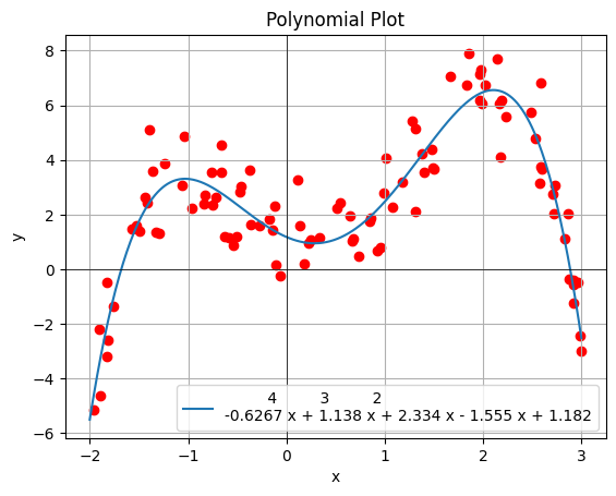
Figure: Plot of the polynomial regression prediction vs. data
We can extend our linear model to be that of a degree m polynomial. In the problem setup we are again given n observations labelled \(X=(X_{1}, X_{2},...,X_{n})\) and n responses \(Y=(Y_{1},Y_{2},...,Y_{n})\). In this case we just have 2 dimensional data where each \((X_{i},Y_{i})\) is a point in the plane. Hence our model is:
Here \(\beta=(\beta_{0},...,\beta_{m})\) are constants that will have to be worked out so the model fits the data well. We again can do this by applying our knowledge of regression. For this specific problem we use least squares as our lost function. So we want to solve:
We can now see that it is the exact same optimisation problem we encountered in linear regression. Remember we are taking the gradient with respect to \(\beta\) so we will have the same matrix as in linear regression but with each column i raised to the ith power (the only difference in the solution are our variables will be raised to a power instead of being all linear). Hence our solution is:
Note again that our loss function is convex so our solution is the minimum and it's unique. We can now move onto coding up our solution and training the model. This time we will randomly generate 100 points between -2 and 3 and, plug them into the polynomial \(1-1.2x+2.4x^2+x^3-0.6x^4\) and then add some noise to the output (noise is generated from a standard normal distribution).
    import random

    data = [random.uniform(-2, 3) for _ in range(100)]

    pol_lis = []

    for i in range(len(data)):
      pol_lis.append(1 - 1.2 * data[i] + 2.4 * data[i]**2 + data[i]**3 - 0.6 * data[i]**4)

    Y = np.array([x + random.gauss(0, 1) for x in pol_lis])
We also change our augmentation function to also raise the data to the power of the i, where i is the column. The rest is the same as linear regression.
  import numpy as np

  m = 4

  def Augmentation(data):
    X = []

    for i in range(len(data)):
      X.append([data[i] ** j for j in range(1, m + 1)])

    X = np.array(X)
    X = np.c_[np.ones(X.shape[0]), X]
    return X

  def Error(X, Y, beta):
    return np.linalg.norm(np.matmul(X, beta) - Y)**2

  def PolynomialRegression(X,Y):
      beta = np.matmul(np.matmul(np.linalg.inv(np.matmul(np.transpose(X), X)), np.transpose(X)), Y)
      return beta


  X = Augmentation(data)
  beta = PolynomialRegression(X,Y)
  error = Error(X, Y, beta)
Running the code we get an error of 105.8, this error comes from the noise we added. Comparing the coeffecients we got to the coeffecients of the polynomial we used to generate the data we see they are very close. This means our polynomial regression was succesful. Also in the colab book is a code sement for viewing plots of the data and prediction line. When we plot them out we see the following graph which confirms our model is succesful at predicting the data.